Imagining undiscovered species with neural networks

TLDR: Neural networks are cool. I trained a recurrent neural network on a list of around 25000 species names and made it generate its own, then built a Twitter bot that tweets one out every hour. The results are kinda funny.

I’ve always been interested in the application of artificial intelligence techniques to ecology. There’s huge potential and some very low hanging fruit in the use of machine learning to make predictions about species distribution and abundance, as well as a whole list of other things like evolutionary processes and taxonomic classification. Generative neural networks can sometimes also produce some surprising and funny results. I see it as a form of uncanny valley, where the results produced are similar enough to be plausible, but strange enough to cause a moment of cognitive disconnect. Koans in AI generated text. These texts give insight into our own lingual and syntactic abilities. What is normal language and what are the rules by which we produce and recognise it? Why is it so funny when those rules are broken?

I was recently inspired and amused after coming across an article on Janelle Shane’s blog, in which she lists recipe names generated by a recurrent neural network trained on a corpus of about 30 000 real recipe titles. Janelle has also turned her neural network to several other text sources, including Irish folk songs, knock knock jokes, Pokemon names, and full recipes themselves, all with hilarious results. I decided that I would take up the torch (you’ll get the pun in a minute) and have a go at producing a neural network capable of generating plausible species names.

Firstly, I needed to gather a training dataset. In order to broaden the appeal and increase the comedic value of the output, I decided producing common names for each species was important, so that meant I needed a dataset of species that had common names. This was a little hard to find. In the end I cobbled together lists of around 12600 animals and 14700 plants from various online datasources including the Atlas of Living Australia and the Global Biodiversity Information Facility. For each species I included the family name, the species binomial, and a list of common names. I kept the plants and the animals separate. The animals dataset was quite heavy in marine creatures, which is visible in the output – the network generates a lot of eels, fish, and crabs.

So how’d I actually do it? And what is ‘training’ a neural network? There’s a very good explanation of how recurrent neural networks work here, although that may be a little technical for most. The simple explanation (and this is about the extent to which I understand it properly, so feel free to update or add to my knowledge in the comments) is this: The neural network looks at each character in the source text at a time, and it makes a guess about what character will come next based on all the previous characters that it has read. Then it checks that next character, and updates its model according to whether it guessed correctly or not. The network doesn’t know anything about english; it doesn’t know anything about the subject matter; it just sees each character as a vector within a probabilistic space and it builds a model around those probabilities. How do you actually train it? That part is pretty simple, thanks to the great tools that have been built in this space over the last few years.

I used torch-rnn, a recurrent neural network package for the Torch (there’s the pun!) scientific computing framework. I followed the excellent guide here, and while I had to dive into Github issues a couple of times to solve installation glitches and even had to modify the source code to run on my machine, I got it up and going within an hour or so. Training took a while on my GPU-less MacBook Air – around 12 hours each for the animal and plant datasets. At the end of that process I issued commands that asked the neural network to generate sets of species names based on the animal and plant models it had developed. The output of these went into a text file ready for my Twitter bot to tweet. I generated enough to keep the bot going for around a year at one tweet per hour.

The results don’t quite have the comedic value of Janelle Shane’s recipe titles, but biologists might find them amusing, and it is really interesting how the AI has learned many of the rules of species naming – that plant families should end with -aceae, and animals with -dae, and that species names should have a ‘latin’ feel to them. In many cases it even used real family names, and sometimes genus names, I guess because there are few enough of them that it could learn that the whole word was commonly used. It learned that species names should be in two parts, and that common names often include hyphens, possessives, and terms like ‘weed’, or might end with ‘fish’ or ‘rose’. Of course, there are many times it gets those things wrong too – sometimes producing a family-like name in place of a species name, which resulted in the bot tweeting a species-like name in place of the common names, or else just combining things in some unrecognisable fashion.

The bot itself is pretty standard; using the Tweepy library really makes it easy to set up a Twitter bot. It runs on my Raspberry Pi, and is triggered by a cron job every hour.

Follow Undiscovered Species on Twitter to keep up with the names.
Privacy in the age of surveillance

At a party recently, someone said ‘Well, this is a conversation we couldn’t have on Facebook’, regarding a tongue in cheek plan for sedition and revolution. I suddenly realised that with the introduction of wearable recording devices, we will not be able to have that conversation anywhere. Most of my friends are already carrying devices that can record everything, it’s just that they’re in pockets or handbags, and we assume that our friends are not surreptitiously recording our conversations, and that those devices are secure and un-hacked by agents of power (in case you don’t know, it’s possible for malicious entities to activate microphone, camera, and gps functions on smart phones remotely to record everything you do, without your knowledge).

It’s already a problem with tagged photos on Facebook, and there have been a few recent incidences when I have requested that photos are not taken or at least don’t go on Facebook, because they could have been compromising for me or other people present. I really don’t need all 500 people on my friends list seeing what I get up to every Saturday night – not that it’s very embarrassing, or illegal – it’s just that when I’m having a good time, I don’t want to have to think about how I look to those on my list that I have a more formal relationship with, or how it might look in 10 years when that photo has become available outside of Facebook, and Google has tagged it with automated facial recognition, and it’s on record for ever. Recent conversations have shown me that many people really just don’t understand the privacy implications of what they do online – and others do, but just have different ideas to me about what’s acceptable and appropriate in terms of documenting and sharing. There are no absolutes, and while I would err on the side of caution when deciding whether to pull out my camera in a questionable situation, others take a different approach. We haven’t yet developed social rules to deal with these questions.

What will happen when Google Glass, or similar technologies become widely available? A quick search for ‘wearable camera’ returned these in the top results:

Narrative
Autographer
MeCam

You can buy these things already. They clip on to your clothing, automatically take photos or videos all day, and upload them to a cloud service. The totally-recorded life is now an affordable reality. I can think of some awesome uses for this, particularly for ecological fieldwork, which is one of my interests. Lost the tag from a specimen and can’t remember where you collected it? Just consult the recording from the camera you were wearing. (An aside: I’m sure managers will also enjoy the ability to more closely monitor the performance of their workers, which is another issue that has both positives and negatives – as a worker, I appreciate having good feedback, which requires good data – but I also resent micromanagement and unnecessary surveillance.)

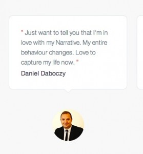
BTW, check out this amazing testimonial on the Narrative site:narrative-testimonial
Apparently his entire behaviour changing is a positive thing.

Narrative have a ‘community‘ – really an Instagram hashtag, with which you can tag the photos it produces as you upload them, to ‘share’ your life with the rest of the internet. Some people have designed beautiful leather holders for their Narrative cameras:

This is the beginning of the wearable computing revolution, and while it will have many amazing benefits, if we continue down the path that we’re on socially and politically, it will also signal the death of privacy completely. It will no longer be possible to have that funny conversation about methods of creating a revolution at 1am on a Sunday morning, because you won’t know who in the room is recording and uploading every word to the databases of the information industrial complex on the pretext of ‘sharing’ their life. We’ve seen several situations where jokes on social media were perceived by authorities as threatening to national security and lead to serious consequences for the poster, so it’s fair to assume that real life instances of similar behaviour will be treated similarly when they are recorded and made public. We are now entering an age where all media is social media, and all socialising (and the rest of life) is recorded and uploaded to cloud services, which are potentially vulnerable to attack by malicious actors (including agencies of nation states), if they are not actively colluding with them.

Another range of wearables, already pretty common, are monitoring biomedical data about ourselves and uploading that to the cloud. Coming soon – devices that are more specific and sensitive:

https://www.indiegogo.com/projects/leo-fitness-intelligence – a system that measures many different parameters to improve fitness activities.
https://www.indiegogo.com/projects/upright-improve-your-posture-and-prevent-back-pain – a device that monitors posture and might reduce back pain.

http://www.wired.com/2014/06/this-cup-tracks-exactly-what-youre-drinking-with-molecular-analysis/ – This is a cup that can tell you what’s in it, including how many calories, and how much caffeine or alcohol. It can tell the difference between 7-Up and Sprite. It can remind you when you are slipping on your diet goals.
https://www.kickstarter.com/projects/892018590/kgoal-smart-kegel-trainer – This is the winner. A device that, when inserted into the vagina, can help the user to improve their pelvic floor strength by monitoring pressure. It gives tactile feedback by vibrating, so you get a little buzz when you squeeze it properly. Of course, it comes with an app that tracks your progress.

Again, the technology is amazing and will no doubt have many benefits, but we’re opening up the insides of our bodies and the tiny details of our daily lives to public scrutiny, and anti-public surveillance, without really ever having a conversation about whether that’s desirable, or how we want to manage it if so.

This is 2014. What is 2024 going to look like? These are the last years in which we can safely assume that at least some of our conversations, public interactions, and private activities are actually private. Enjoy it. And let’s talk about what we want to see in this space, and how we’re going to achieve it, before we all get distracted by the shiny new iWatch or Android EEG monitor, or whatever comes next.

Heatmap of Threatened Plant Species of Australia

Using data from the Atlas of Living Australia and tools from Mapbox, I created a heatmap of observations of threatened plant species in Australia.

Methods

Preparing the data

I accessed the ALA’s excellent web services API to get the data on threatened plant species observations. I wrote two python scripts to gather this data; the first got the GUIDs (a unique ID) of each plant species that had a Commonwealth conservation status of Rare, Vulnerable, Endangered, or Critically Endangered. Once I had all those GUIDs (around 4000 of them), I ran the second python script which queried the API for all observation records for each GUID (sorry for the server hit, ALA!). Once I had all those observations, I simply stripped the location coordinates out of them, as I didn’t need to know anything more about them for this project, and then wrote the coordinates to a csv file. The result was 11086 coordinates.

Making the map

I loaded up QGIS and imported the csv of coordinates. Following these instructions, I built a heatmap from the coordinate points using a 100 km radius (meaning that the map shows numbers of other records within 100 km) and the Triweight kernel shape. I used a cell size of 0.1 map units (ie, degrees, since I was running this project in WGS84), which I figured would give good enough spatial resolution while keeping file size reasonable for upload. Many of the records I was working with were generalised to 0.1 degrees anyway, in order to protect the exact locations of the conservation-dependent plant species. In order to get the map onto the web, I used Mapbox’s TileMill software. I exported the heatmap from QGIS, reprojecting the image into Google Mercator projection (900913) to make it display properly in TileMill. From TileMill, I uploaded the map into my Mapbox account – and here it is.

Results and Discussion

The Map

Explanation

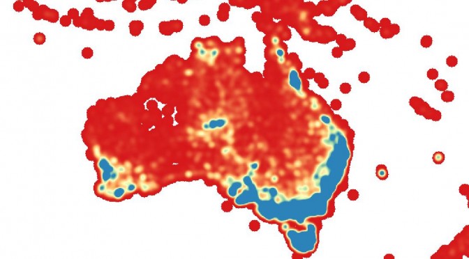
The legend doesn’t show up in the embedded map, but you can see it in the full map. Here’s an explanation of what the colours actually mean. The numbers displayed in the legend are increments from 0 – 5.69 (roughly). The values refer to the number of records of threatened plant species observations within a 100 km radius of any spot. In the red sections, there were no other records within 100 km (ie there was only one record). In the blue sections, there were at least five other records within 100 km of the cell. The numbers were calculated based on the estimate cumulative cut of the full extent of the map (which may have been the wrong method to use – see below), using a cut value of 2 – 98%.

Discussion

The pattern shown is that the known biodiversity hotspots tend to be blue coloured. This explains the blue in the south west corner, in the area between Melbourne and Adelaide, in Tasmania, and in central Queensland. That’s not a surprise. But this analysis was based on numbers of records, not necessarily numbers of species, and it was based on threatened species only, so there’s some other factors that affect the appearance of the map apart from biodiversity.

The first is survey effort. Areas closest to populated parts of the continent are, by default, likely to be more frequently visited by ecologists, recording observations of species. This explains the heavy blue colour up the east coast, where most of Australia’s population is concentrated. This factor may also explain the high values around Alice Springs in central Australia, Darwin, and Townsville in Queensland, which are not known as biodiversity hotspots, but where research institutions such as herbaria and universities are based, which allow increased recording of data. Survey effort (or lack thereof) may also explain the lack of many records in some areas that are known biodiversity hotspots – for instance, the Kimberley in WA, and to a lesser extent the Pilbara – which does have a faint orange/yellow colour, and which has been relatively highly surveyed due to environmental consultants carrying out environmental impact assessment surveys for the booming mining industry over the past ten years. For that reason, my expectation was that there would be more records in the Pilbara – but there are only a couple of Commonwealth-listed threatened species from the area, which probably explains it. High biodiversity doesn’t necessarily equate to large numbers of threatened species, either for entirely natural reasons, or because of delays in the reporting of data (which are quite likely to be a major contributing factor).

The final factor that may complicate things is that this study looked at threatened species. Therefore, it is likely that there will be more records in areas that have been highly disturbed, such as urban and agricultural areas, because due to Australia’s high rate of endemism, there are many species that only occur within small geographic areas, and when those areas have been heavily modified, it’s likely that those species will have become threatened. Again though, this theory fails to explain the lack of records in the Pilbara, an area that has been heavily disturbed by mining and grazing.

Limitations

Map colours

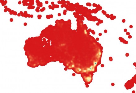
I wasn’t sure if the method I used to colour the raster image was the most appropriate. The main problem with this method is it fails to discriminate between pixels with higher values. The maximum value present in the raster was 81.977, which is considerably higher than five, which is the value at which the colours stop changing. This means that, although there are relatively few data points at these high levels (the mean value was 1.263, and standard deviation 4.763), the large range is all squished into that one colour. This could potentially hide areas of unusually high threatened species records.

In order to test this, I recoloured the map using the maximum and minimum values rather than the 2-98% cut, and using the actual, rather than estimated values, which takes a little longer (although the difference is negligible for this map), but results in the true (higher) value for the maximum. I also changed the colour increments from continuous (which defaulted to five colour classes) to incremental, and manually specified ten colour classes. The result looked like this:

Result of recolouring raster image with maximum value and ten colour classes

As you can see, this is effective at highlighting the areas of really high observation numbers, however it too has a downside – the vast majority of pixels are now classified at the lowest levels, which means the main body of the variation in the map is invisible.

One solution to this problem is to manually modify the colour breakdown to produce the most visually clear and expressive map. I played around with this, and managed to develop a map which appeared to differentiate between the large number of pixels at the lower end of the spectrum, while allowing those few pixels at the very high end to stand out as highlights. The only downside to this is that it’s a very subjective process. I wanted the map coloration to have a clear mathematical relationship with the data, even if that meant losing a little bit of detail at the top end. For that reason, I stuck with the original method.

Why does Tasmania look so weird?

I don’t know. I think it must be a problem in the process of TileMill creating png map tiles out of the GeoTIFF raster. It’s not present in the raster in QGIS, and it’s not visible at all zoom scales in the TileMill map.

Displaying Django form field help text in a Bootstrap 3 Popover

Bootstrap and Django make a great combination; but sometimes it’s a little tricky to integrate them in a neat way.

I like to display form field help text in a tooltip-like element in my web forms. In Django models, help text can be defined as a field attribute called help_text. I want this text to appear in a tooltip when the user hovers the mouse over the form field.

Previously, I’ve used the amazing and very powerful qTip2 for this, but since I’ve already got the Bootstrap libraries in my project, which come with a good tooltip plugin called Popover, I figured that I could get by without including another javascript library. Displaying help text is a simple function that doesn’t require the advanced customisability of qTip2.

The Bootstrap 3 popover can read the following attributes present on the element the popover is attached to:

  • data-container="body": The popover will function without this, but it might display weirdly, so better to include it.
  • data-toggle="popover": This is not essential if you bind the popover to the HTML class as I’m doing below.
  • data-placement="left", or right, top, or bottom. Determines where the popover appears in relation to the anchor element.
  • data-content="The text you want to appear in the popover."

In order for these elements to get into the HTML of the Django form field, we need to modify the attrs attribute of the field’s widget. Here’s how you do it in the form class:

class ItemForm(forms.ModelForm):
    class Meta:
        model = Item

    def __init__(self, *args, **kwargs):
        super(ItemForm, self).__init__(*args, **kwargs)
        for field in self.fields:
            help_text = self.fields[field].help_text
            self.fields[field].help_text = None
            if help_text != '':
                self.fields[field].widget.attrs.update({'class':'has-popover', 'data-content':help_text, 'data-placement':'right', 'data-container':'body'})

As you can see, after calling the __init__ method of the parent class, we loop through the fields in the form and assign the help text to a local variable. I’ve then chosen to assign the help_text attribute on the field to None, because I don’t want it showing up in my form elsewhere, but you may want to keep it, particularly if you are customising your form’s HTML in the template. For those fields that had some text in their help_text attribute, we then update the widget’s HTML attributes to include the data necessary for the popover to function. The has-popover class gets added so that we can identify these elements on the template and initialise the popover javascript on them.

The javascript in the template then looks like this (of course the bootstrap javascript library has already been called somewhere):

$(document).ready(function() {
	$('.has-popover').popover({'trigger':'hover'});
});

I want my popovers to appear on hover, rather than on click which is the default, so I’ve specified that as an option in the popover initialisation.

And there it is – you should now have a functional bootstrap popover on your form field.
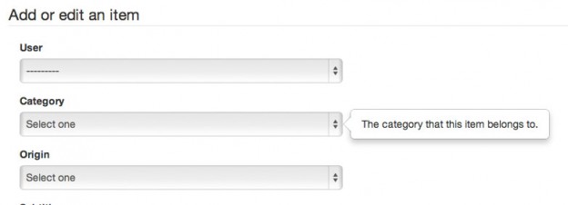
Here’s mine:
popover-grab

Note – this works for a model form, but in a normal form, you could easily specify the same attributes in your manually described field instances.

Note 2 – Some people may consider that putting HTML attributes into the form __init__ violates MVC principles, and it would be better to add these attributes in the template itself. I have done so in the past, using qTip2, however that requires more HTML and much more javascript, and I find this to be an overall neater solution. If you don’t initialise the popover, those additional attributes don’t do anything by themselves and only add a very small load to the browser. Django widgets are designed to allow modification of HTML, and it makes sense for me to take advantage of this capability because I use Bootstrap in tight coupling with my Django setup. I am very open to suggestions of people doing something similar in a different way, though – please comment :).

Spring Orchids

The first orchids of spring have started blooming in the south west. I’ve just spent the weekend out botanising with some adventurous friends to see what we could find near Margaret River. First stop was to see the Meelup Mallee (Eucalyptus phylacis), a 6600 year old clonal individual tree growing near Dunsborough. After walking around at the site for some time, we realised that we were actually walking amongst the stands of the tree, which consists of 26 ramets (separate but genetically identical ‘clones’). Many of these ramets are separated by tens of metres, and the other jarrah woodland species are abundant in between, so it is not easy to recognise that these stands are actually parts of the same organism. Considering that there is such distance between the stands, and they do not produce viable seed, the only way this individual could have spread across such a large area would be vegetatively, and hence it must be very old. The mallee is fascinating, but not particularly visually exciting, so I did a bit of orchid hunting in the area for photographic interest. I found a very pretty Caladenia reptans subsp. reptans.

Caladenia reptans subsp. reptans orchid flowers
A relatively common orchid species found in the south west

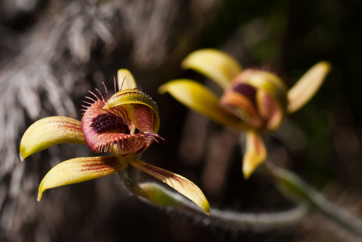
Next stop was the habitat of a species called Caladenia caesarea subsp. maritima, which grows only in granite outcrops along the coast near Busselton. There are only six known populations of this species, and approximately 650 individuals. It is listed as Threatened (Declared Rare) Flora in Western Australia, and ranked as Endangered under the Commonwealth legislation (more info here, FloraBase page here). After some time spent poking around amongst the rocks (during which we found some Cyrtostylis huegelii growing under a small granite boulder), we finally found the Caladenia – although only two plants, one with a single flower, and one with two.

Caladenia caesarea subsp. maritima orchid flower
Caladenia caesarea subsp. maritima, a Threatened orchid species in Western Australia

We were so excited about the orchid, and engrossed in taking photos of it, that we failed to notice several humpback whales playing in the bay only about 100m away from us. When we finally saw them, we ran down to the water and enjoyed watching the whales for an hour or so; unfortunately I was not able to get many good photos – every time a whale raised a fin I was unprepared and by the time I had focused, the whale had gone back to appearing as a dark patch of water in the photos. This is the best I could do:

A whale in Geographe Bay

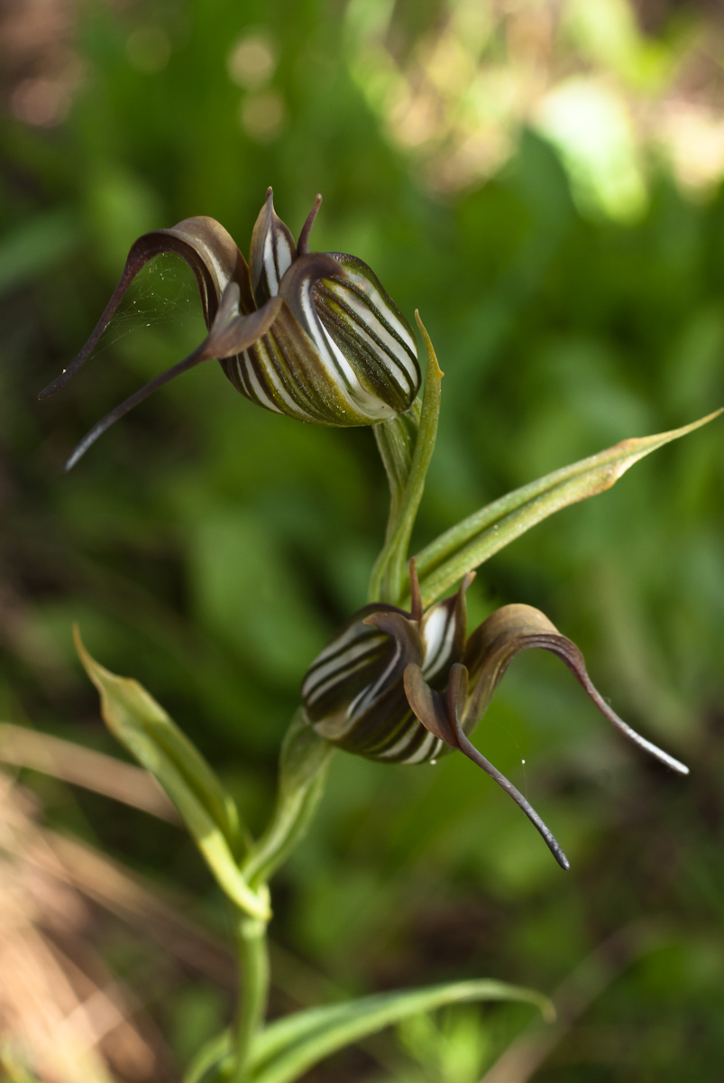
After that excitement, it was time to get some supplies from Margaret River and set up camp at Contos. The following day we drove to Boranup forest to enjoy the views and climb some Karri trees. While we ran out of time for tree climbing, I did find some snail orchids (Pterostylis something, probably P. pyramidalis):

Snail orchid flowers
Snail orchid (Pterostylis species)

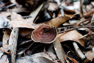
I also found this fungus, one of my favourite looking species, Coltricia oblectans

Coltricia oblectans fungus
Coltricia oblectans

.
The weekend continued with some rock climbing at Wilyabrup – and all round was the most fun I have had in a short space of time for a long time.

Cliffs over the ocean at Wilyabrup, south of Yallingup
Cliffs over the ocean at Wilyabrup

Pilbara Adventures

Definitely long overdue for an update. While I have a few things to catch up with from late last year, I’ve recently spent some time botanising in the Pilbara; near Newman and Port Hedland, and I’ll post about the Newman work now.

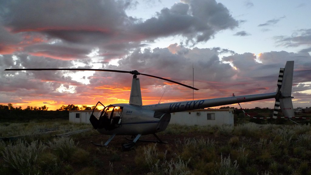
I spent a couple of weeks working near Newman, spread over two periods in November last year and March this year. Both jobs were flora surveys for mining proposals, and both jobs involved the use of a helicopter. I was quite excited about this at first, however the fun soon wore off. The helicopter was small, cramped, difficult to get in and out of, hot, noisy, and imparted a sense of hurry to the work which I didn’t enjoy, due to the fact that the pilot would often leave the engine and rotors running while waiting for me to finish off a site.

helicopter at sunrise

Another day begins

It was a great way to experience the landscape though, and to be able to see changes in vegetation types from above made the work easier. Every landscape has its optimal viewing distance for maximum visual beauty; and the stony hills of the Pilbara are best suited to being seen from about 100m up.

Stony hillsides with creeklines are common land forms in this part of the Pilbara

Being in the helicopter also enabled me to get an interesting (and sometimes slightly scary) angle on the weather. On most days our work was cut short by the development of thunderstorm cells, and several times we dodged around active thundersorms on our afternoon commute back to our camp.

Thunderstorms from the air

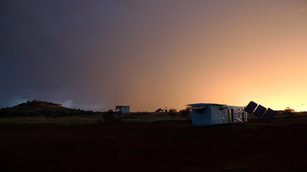
The weather was also interesting to photograph from the ground. This is the sky after a storm passed over us at Sylvania Station, where we camped:

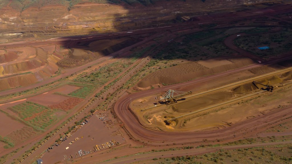
While flying in the helicopter, it was interesting to note the number and extent of mining activities in this part of the country, which was mind boggling. Our daily commute took about an hour, and in this time we would pass over three active mines and several areas of development that appeared to be planned mines, as well as various camps and other infrastructure such as railways and roads.  It seemed that there was some kind of construction project happening in every valley. If there was no major developments, then there would at least be drill pads on the ridges and sometimes the flats.

Mining landscape

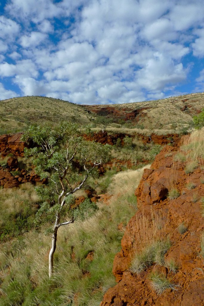
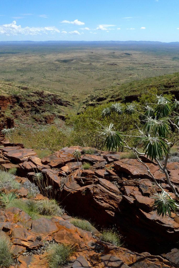
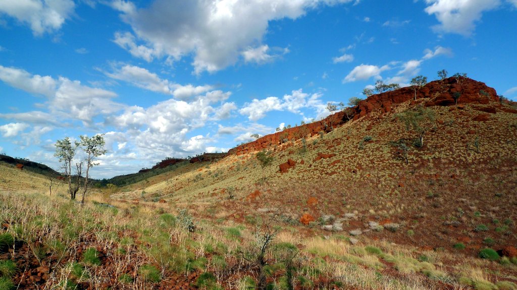
The area north of Newman is known for its stony hills, gorges (exemplified by those at Karijini National Park), and open plains dissected by sandy creeks. The vegetation is ‘spinifex’ Triodia grasses with Acacia shrubs and/or sparse small Eucalyptus trees. Members of the Malvaceae (mallow) family are common shrubs; as are peas.

 Typical Pilbara landscape

View from above. Iron plant (Astrotricha hamptonii) in foreground.

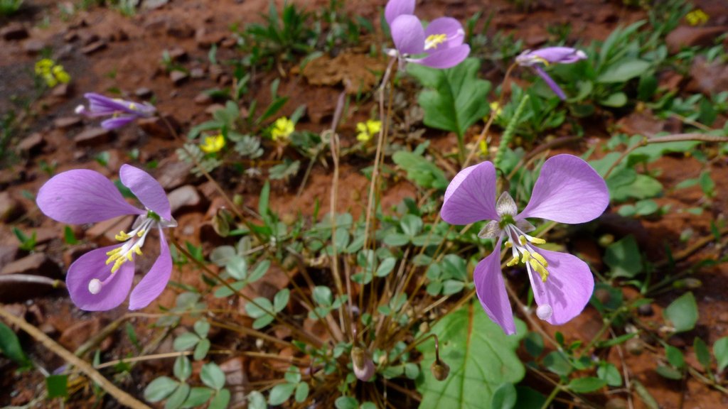
The pretty Cleome oxalidea occurred on clay flats in the area

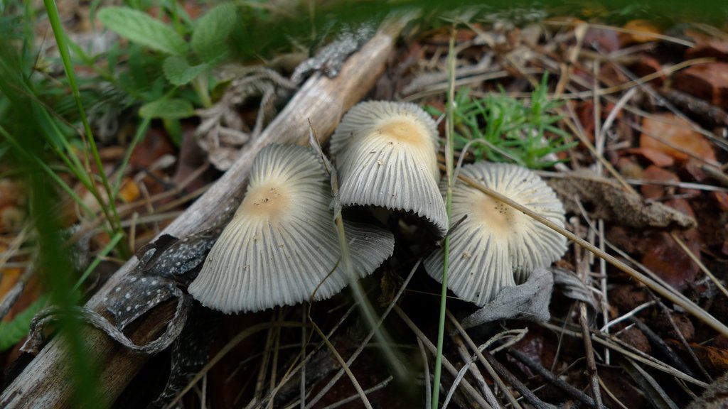
I also encountered some mushrooms, both unusual for this area from my experience. An Amanita, found emerging from a rocky hillside, with an unusual double annulus:

And a Coprinus, or related genus, found in a dense creekline:

And a final landscape:

Spring Wildflowers – Part 1

It’s still early spring, but the orchid season is in full swing in the South West. Although I haven’t been able to explore far afield yet, a few short walks have yielded an amazing number of species. I counted eight species of orchids in a short walk around Wireless Hill park in Applecross last week – most of the below photos are from this location. This may be due to the ‘near average’ rainfall – the best that Perth has had in ten years (BoM Winter Rainfall Summary).


View Larger Map

Wireless Hill is itself an interesting place and has plenty of history. It was known as ‘Yagan’s lookout’, Yagan being the well known indigenous leader and freedom fighter in the early days of the Swan River Colony, whose story is one of the foundational parables of Noongar/White relations in Western Australia. The hill gets an excellent view both west towards Fremantle and north-east towards Perth and was obviously of some strategic importance for that reason.

There is currently a very active Friends Group who can be observed (or assisted) in looking after the bush. There are significant ecological problems as there usually are in small urban remnant bushlands; especially weed invasion, and frequent fire. However, the Friends group is actively removing the weeds, and in some areas, I was greatly impressed by the health of the native vegetation, no doubt due to their hard work. They host a list (Microsoft Word .doc file) of the flora that have been recorded there.


This beautiful group of Caladenia discoidea, the Dancing Orchid, was found at Wireless Hill. I was excited to see these as I had never seen this species before.


Another shot of Caladenia discoidea flowers. This species is characterised by its short petals and flattened, disc-like labellum. There are often stripes on the petals, and the petal colour is variable, ranging between yellow, white, and pinkish.


A Jug Orchid, Pterostylis recurva.

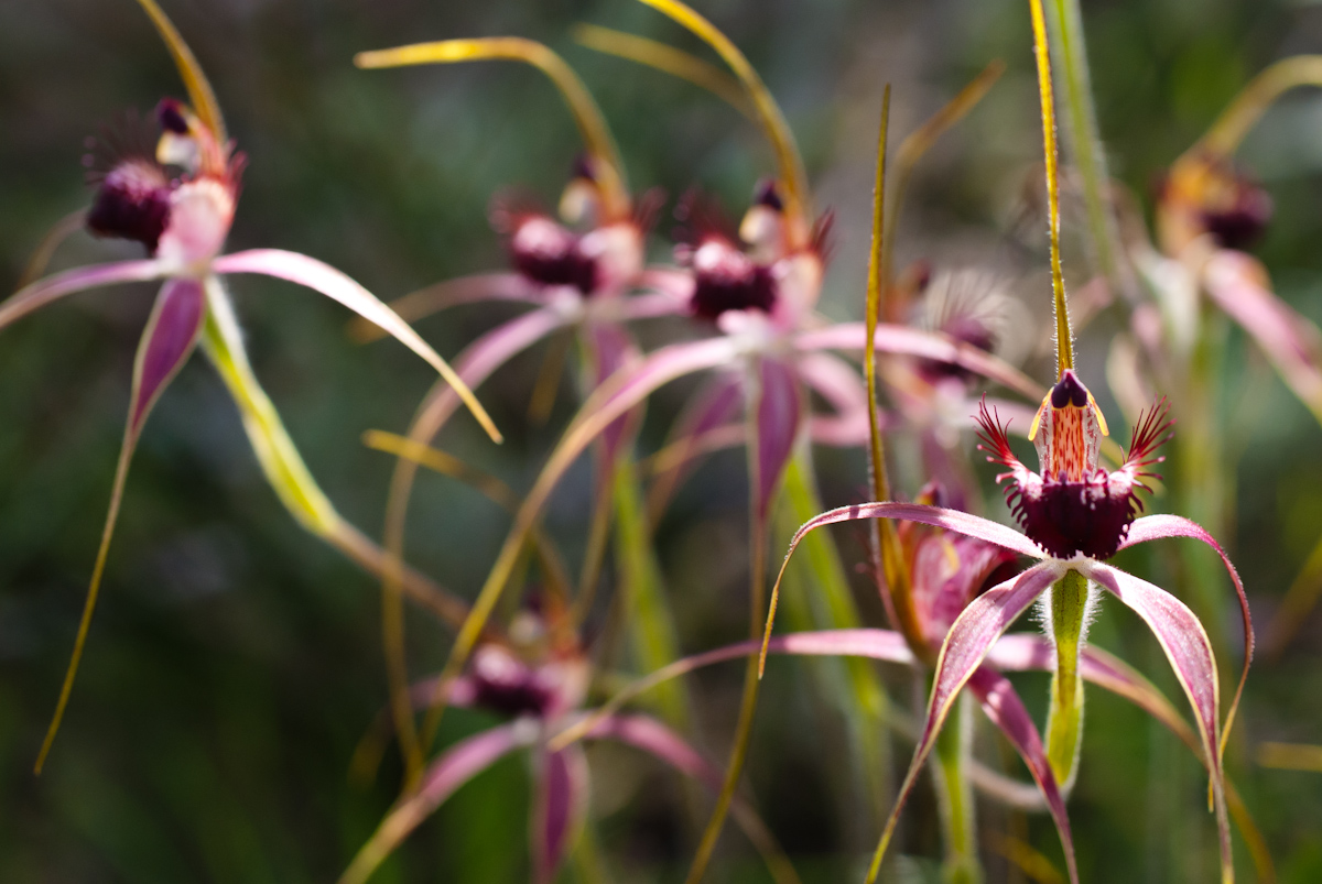
Caladenia arenicola
The Carousel Spider Orchid, Caladenia arenicola. The specific epithet means ‘from sand’, indicating this species grows on sandplain country. Wireless Hill is also host to several other spider orchids; I saw Caladenia longicauda on the day I visited, and the very rare and very large Grand Spider Orchid, Caladenia huegelii has also been recorded there.


Although maybe not as exotic and fascinating as the orchids, Anigozanthus manglesii is quite spectacular and is the flora emblem of our state. I have rarely seen them as healthy and as numerous (except in horticulture) as I saw them recently at Wireless Hill.

Pink fairy orchid
The Pink Fairy Orchid, Caladenia reptans subsp. reptans, found at a farm in the Capercup area of the south west, between Collie and Kojonup, growing in Wandoo woodland habitat.

I’ll follow up this post with further updates as the wildflower season progresses; it’s going to be a good one. My next trip is out to the goldfields, north of Southern Cross, so I hope to capture some of the beauty of the dry country.

Prints for sale – Fundraiser for the Secoya people of Ecuador

In 2009 I took this photograph of Delfin Payaguaje, grandfather of the family that hosted me, preparing medicinal plants.


Secoya man Delfin Payaguaje, preparing medicinal plats

In order to say thanks, I am selling prints of this image, and donating 100% of the profits to Delfin’s family. The money will help fund the Secoya’s conservation foundation, which aims to protect their land from oil exploration and illegal logging. The Secoya are also planning an ecotourism business, which is well organised and nearly ready to go. They have some excellent facilities; but they just need a bit more seed funding to finish building the infrastructure. $1000 USD will make a huge difference to them, and may be enough to launch their tourism operation. If I can sell a few more prints, I will be able to send them a thousand dollars.

The prints are 16″ x 24″ inches (the images are slightly smaller, because there is a bit of white space around them), on high quality photographic paper. I will be printing a limited edition run of ten signed copies.

I am asking for $250 for an unframed print, and $400 for a framed print (all prices are in AUD). The frames are simple black wood, with high quality acid-free matting. I can post unframed prints within Australia, included in the $250 cost; if you want me to send you a framed copy, I am happy to do so but I would like you to cover the additional cost. I can send prints framed or unframed internationally, however will need buyers to cover the cost of postage so that I can send the maximum amount to the Secoya.

I have sold two three of the ten prints so far, and I would like to send the money by October 17 2011. This means I will be taking orders for prints until October 10. Please contact me to place an order.

Thanks a lot for reading; if you’d like to read more details about this project, and the story of my time with the Secoya, please see this post.

Staying with the Secoya – Part 2

Just a reminder: please go back and read the first post in this series if you haven’t already – I’m selling prints of one of my photos and donating all profits to the Secoya people of Ecuador in order to help them raise money for their conservation fund and ecotourism business.

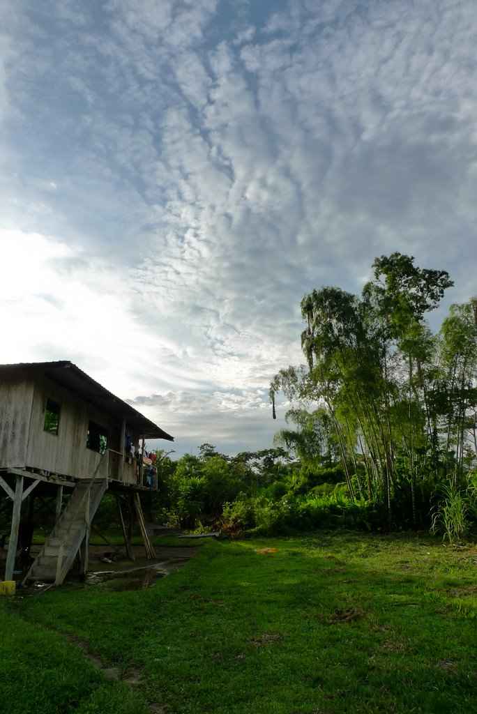
House in the jungle
A typical ‘zinc house’ of the Secoya. All of the timber for the house is cut with chainsaws. The house is called a zinc house because of the metal sheeting on the roof, as opposed to the palm frond thatched roof of the traditional buildings of the Secoya. This PhD thesis by Gabriel Arboleda is an excellent exploration of Secoya building styles and how they have been affected by cultural change before and since colonisation.

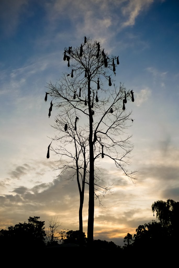
Tree with many hanging birds' nests in it against the sky
These birds nests hang from many trees in the clearings around the village of San Pablo and elsewhere in the upper Amazon. We called them ‘droopy nest birds’, but the Secoya called them caciques, a Spanish word for ‘chief’.

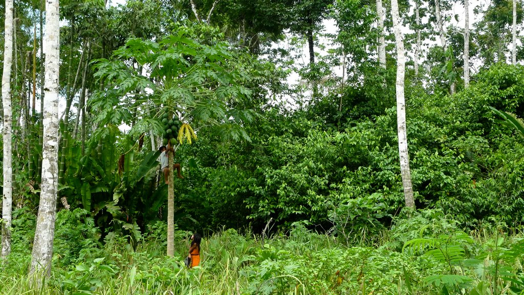
Secoya kids climbing a tree to harvest papaya fruit
Secoya children from the family we stayed with collecting papaya fruit from a tree in the rice paddy.

Secoya man harvesting rice
René, one of our hosts, harvesting rice from their dryland paddy.

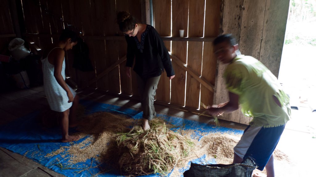
People threshing rice with their feet
Georgia along with René and Lidia Payaguaje threshing the rice that was harvested that day.


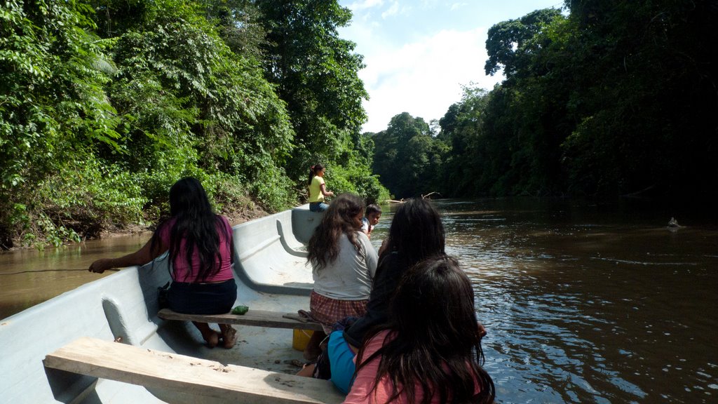
Every boat trip is an opportunity for some fishing in the Rio Aguarico.

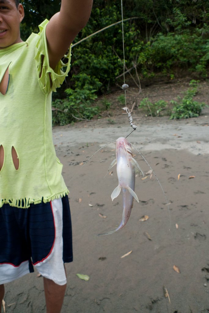
A catfish on the end of a line, pulled from the river
René with a catfish he had just caught from the river.

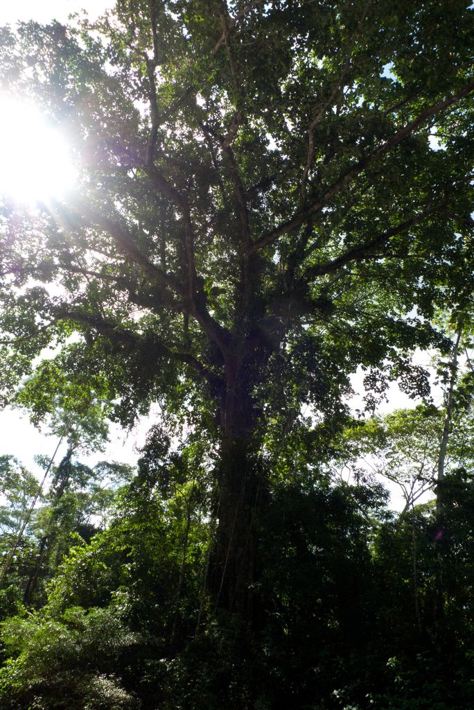
A giant tree overhanging the river
A giant tree overhanging the river.

Part three of this series will focus on the biology of the rainforest – plenty of plants, animals, and weird fungi.